Constrained Least Squares Problem

Solving the 1/2 nonnegative equality constraint

Table of Contents

• Overview
• Background Research
• Steps
• Results
• Conclusions
• References
• Thank you

---

Overview

image of Christian on the whiteboard

My first impression of the problem is that it should be simple to ensure all the weights (theta) are nonnegative but I wasn’t quite sure how to ensure half or less of the parameters end up nonnegative, mainly because I didn’t know which half of the parameters I should constrain. At that time, I was also not familiar with projected gradient descent under different constraints. But by the end of this exercise, I feel much more comfortable in dealing with these sort of constrained optimization problems. But I obviously have a long way to go on the topic.

I understand that I did not solve the problem in the hour allotted but I wanted to ensure that it is clear that I can solve a problem on my feet and as you can see here and here, I am continuously working on my mathematics for machine learning and is also why I’ve begun writing a mathematics book, titled, Mathematics of Deep Learning; as a way to solidify what I do know and extend myself where I don’t.

Here, I will try to give you a quick outline of my background research on the matter to convey my understanding and the results to complete the problem with constraints

Problem Formulation

Our typical case is the least squares case which can be detonated as

\[{\displaystyle \operatorname {arg\,min} \limits _{\mathbf {x} }\|\mathbf {Ax} -\mathbf {y} \|_{2}}\]

in the linear case. This is straightforward but what we’d like to do here is add a constraint that ensures that half of the parameters are nonnegative. \[subject\ to\ x ≥ 0\] (Where x is half of the parameters) We want to find the feasible set that fits our constraint.

We could add regularization but this would only resolve the issue softly. If we want half of the parameters to be constrained to be nonnegative, then we are dealing with a hard constraint so the projected method is one of the better approaches and is also the constraint in need of satisfying.

Background Research

The most basic idea I had was to use a similar method called non-negative least squares which I was only slightly familiar with. I am not currently well studied in operations research nor constrained optimization so I had to study up, which I am happy to do but thought I should make this clear. Here are some of the topics I found myself reading in response to the task

• sub-gradient method
• quadratic programming
• nonnegative least squares
• projected gradient method
• alternating projected gradient method
• fast coordinate descent
• semidefinite programming
• interior points
• Karush–Kuhn–Tucker (KKT) conditions

Steps

I will now walk through the steps I took to arrive at an early solution that meets our constraints.

1. NNLS (try something familiar)
2. Projected sub-gradient
3. Alternating projected subgradient
4. Implementation with unique constraints

Nonnegative least squares

\[{\displaystyle \operatorname {arg\,min} \limits _{\mathbf {x} }\|\mathbf {Ax} -\mathbf {y} \|_{2}}\] \[subject\ to\ x ≥ 0\]

Nonnegative least squares (NNLS) is said to be equivalent to quadratic programming, it takes the least squares method and adds the constraint that every value in x (coefficients) needs to be nonnegative (x >= 0).

\[{\displaystyle \operatorname {arg\,min} \limits _{\mathbf {x\geq 0} }\left({\frac {1}{2}}\mathbf {x} ^{\mathsf {T}}\mathbf {Q} \mathbf {x} +\mathbf {c} ^{\mathsf {T}}\mathbf {x} \right),}\]

NNLS has been shown to be comparable to the LASSO method in regards to prediction without using explicit regularization.

Here is my implementation using the projection method to achieve nonnegative least squares.

 
import numpy as np
X = np.random.rand(10,10)
y = X*2
n,m = X.shape
theta = np.random.normal(n, m, (n,m))
alpha = 0.005
bias = 2
half_obs = m*n/2
cost = 0

def input(X, y, iters):
    Xt = X.transpose()
    gd(Xt, y, theta, alpha, m, iters)
    
def gd(x, y, theta, alpha, m, iterations):
    xTrans = x.transpose()
    for i in range(0, iterations):
        y_hat = np.dot(x, theta)
        loss = y_hat - y
    
        cost = np.sum(loss ** 2) / (2 * m)
        if(i % 1000 == 0):
            print("Epoch %d - Cost: %f" % (i, cost))

# .     take the gradient    
        gradient = np.dot(xTrans, loss) / m
# .     update theta    
        theta = (theta - alpha * gradient)
#       project on to theta and truncate
        theta[theta < 0] = 0
    
    return theta    

input(X, y, 10000)

Epoch 0 - Cost: 14975.095790
Epoch 1000 - Cost: 10.810520
Epoch 2000 - Cost: 2.548314
Epoch 3000 - Cost: 1.522140
Epoch 4000 - Cost: 1.130509
Epoch 5000 - Cost: 0.963231
Epoch 6000 - Cost: 0.877475
Epoch 7000 - Cost: 0.836454
Epoch 8000 - Cost: 0.812410
Epoch 9000 - Cost: 0.798912

NNLS converges optimally here.

Blue is constrained least squares red is unconstrained least squares

Now how do I apply this to half the parameters and what is this projection all about?

Gradient Projection Methods

Image from math.stackexchange.com

Gradient projection methods allow us to solve constrained optimization problems much quicker than alternative solutions. The projection methods enable us to make large changes to the working set at each iteration, unlike other constrained methods that may only be able to impose one constraint per iteration.

\[P[xk−α∇f(xk)],α≥0,\]

The gradient projection method is guaranteed to identify the active set at a solution in a finite number of iterations. After it has identified the correct active set, the gradient-projection algorithm reduces to the steepest-descent algorithm on the subspace of free variables. As a result, this method is invariably used in conjunction with other methods with faster rates of convergence.

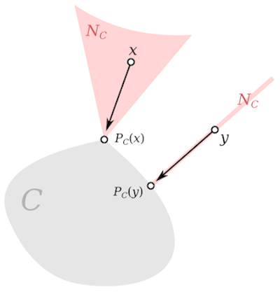
Alternating projections method

\[f(x) = max\ (i=1,...,\ m)\ dist(x, Ci)\]

The alternating projected method generally finds the point where 2 or more convex sets intersect (if they don’t intercept then the method finds the hyperplane between the sets converging towards x* and y*).

They have been traced back to Neumann who said "where the alternating projection between two closed subspaces of a Hilbert space is guaranteed to globally converge to an intersection point of the two subspaces if they intersect non-trivially*[8].

Much earlier work on this method showed linear convergence rates and have been further extended with updated versions (i.e. Dykstra’s projection algorithm, fast projection algorithm, cyclic projection method). It also isn’t the case that x, y need be convex as noted above and some guarantees are still offered.

Here are the steps for projected gradient descent

1. Do a gradient update and ignore any of the constraints
2. Project the result back on the feasible set based on constraints
3. Replace/truncate entries

Implementation with unique constraints

Here are the steps we’ll use for our problem 1. Do a gradient update (ignore any of the constraints) 2. Project unto the half of the result (back on the feasible set based on constraints) 3. Replace/Truncate entries down to zero

Remember that our single constraint is to project on to the first 50% of components to derive the feasible set and ignore the other parameters.

\[theta >= 0, i = [1, . . . ,\ m/2] \]

So now we’ll move into Python to solve the issue and plot the results

Results

Results for constrained least squares meeting problem constraints

Results for constrained least squares

Results for constrained least squares

Python Code

import numpy as np

X = np.random.rand(100,100)
y = X*2
n,m = X.shape
theta = np.random.normal(n, m, (n,m))
alpha = 0.005
bias = 2
half_obs = m*n/2
cost = 0


def input(X, y, iterations, project):
    Xt = X.transpose()
    results = gd(Xt, y, theta, alpha, m, iterations, project)
#     return results

    
def gd(x, y, theta, alpha, m, iterations, project=False):
    xTrans = x.transpose()
    n,m = X.shape
    half_obs = int(m*n/2)
    cost = 0
    
    for i in range(0, iterations):
        y_hat = np.dot(x, theta)
        loss = y_hat - y
        
        cost = np.sum(loss ** 2) / (2 * m)

        # take gradient and update theta
        gradient = np.dot(xTrans, loss) / m
        theta = theta - alpha * gradient
        
        # project and truncate values
        
        theta[(theta < 0).nonzero()[0][:half_obs]] = 0
        
        
        if(i % 1000 == 0):
            print("Iteration %f | Cost: %f" % (i, cost))
            
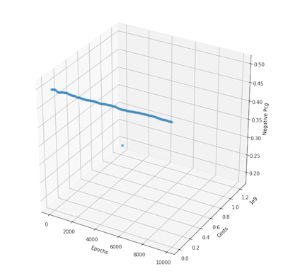
            pcg_negs =  (np.count_nonzero(theta[:half_obs]<0) / (m*n))             
            print("Pcg of negatives %f" % (pcg_negs))     

        
    return({'theta': theta, 'cost' : cost})      

input(X, y, 10000, True)

Iteration 0.000000 | Cost: 1250700514.525059
Pcg of negatives 0.000000
Iteration 1000.000000 | Cost: 16.587968
Pcg of negatives 0.000000
Iteration 2000.000000 | Cost: 16.708769
Pcg of negatives 0.000000
Iteration 3000.000000 | Cost: 17.062254
Pcg of negatives 0.000000
Iteration 4000.000000 | Cost: 17.651817
Pcg of negatives 0.000000
Iteration 5000.000000 | Cost: 17.689826
Pcg of negatives 0.000000
Iteration 6000.000000 | Cost: 17.672136
Pcg of negatives 0.000000
Iteration 7000.000000 | Cost: 17.663930
Pcg of negatives 0.000000
Iteration 8000.000000 | Cost: 17.666040
Pcg of negatives 0.000000
Iteration 9000.000000 | Cost: 17.462005
Pcg of negatives 0.000000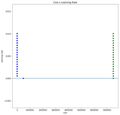

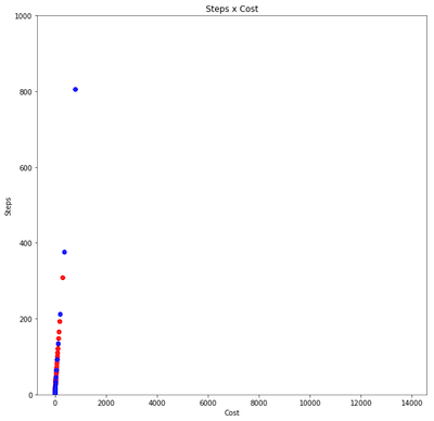
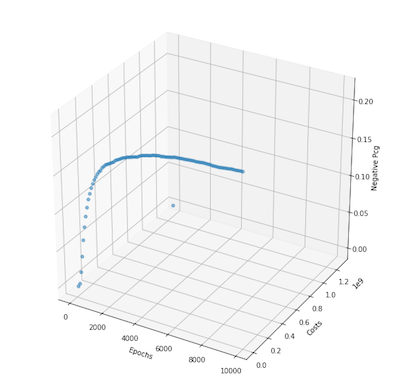
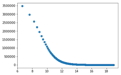
Cost of both constrained and unconstrained methods over different learning rates

• When learning rates are small and the function is simple, the alternating projection seems to converge to the minimum
  
• 10,000 iterations are too little for more complex functions as it takes the projection method longer to converge and sometimes doesn’t converge within the given iterations
• The percentage of negatives is typically stable on problems I tested > 10000x10000 with learning rate between .005 - .001

Conclusions

It took quite a lot of research to find a rather simple technique but the early results after using projected gradient descent with the given constrained met the constraints without a significant increase in the loss when low learning rates are used. It should be noted that the method is extremely slow as theta grows (1000x1000) but could be further optimized with a different projection approach that makes use of shortcuts via linear algebra but would require more time and understanding.

I was excited to explore this subject to complete the challenge and would like to still be considered. As you probably know from my profile, I’m continuing to push forward in becoming what I need to be to become a deep learning researcher to help advance certain aspects of machine intelligence.

Email: thechristianramsey@gmail.com

Other Solutions

In the time allotted I was not able to follow through with many of the trajectories I would have liked to follow. Here would be some of my explorations.

1. Alternating projections on the HalfSpace
2. Use KKT to verify a condition
3. Use bounded-variable least squares (BVLS)
4. Truncate with different values replacement values (although the literature tells us anything from 0 to 1 should be insignificant)
5. Try different sets to constrain
6. Plot contours to better explain method intuitively
7. Averaging over projections?

Alternating Projections on the Half Space

1. Calculate gradient
2. Project into the HalfSpace with our constraints
3. Update theta

References

• Alternating Projections

• Semidefinite Programming

• Positive Semidefinite Matrix

• Projected Gradient Methods for Non-negative Matrix Factorization

• Non-negative Least Squares

• Karush–Kuhn–Tucker conditions

• Ground-motion prediction equations

• Convergence Analysis of Alternating Nonconvex Projections

• Functional operators - The geometry of orthogonal spaces

Thank you